Rural household income mobility in the people’s commune period
The case of Dongbeili production team in Shanxi province
作者:Yingwei Huang(黄英伟,中国社会科学院经济研究所)
Jun Li(中国农业大学经济与管理学院)
Zheng Gu(中国农业大学经济与管理学院)
来源:《China Agricultural Economic Review》,Vol. 8 Iss 4 pp. 595 - 612
摘要:【Abstract】Purpose – The purpose of this paper is to investigate the long-term differences in household income and their causes in the people’s commune through a panel of micro-data. Design/methodology/approach – The income mobility method (including static Gini mobility and dynamic income transition matrix) as well as the multinomial logit model) are employed in this paper. Findings – Empirical results indicate that differences in household income were relatively low during the people’s commune period. In addition, both Gini mobility and income transition matrix analyses show that income mobility in the long term was faster than that in the short term, suggesting income mobility was beneficial for low-income earners in the long term, i.e., there was an pro-poorness. The major factor influencing household income was the structure of family population, not the quantity of labor input. Originality/value – This paper is the first using income mobility method to study farmers’ income disparity and conducting factor decomposition on it in the people’s commune period. The micro-data on production team level applied in the paper is of high value, and the paper is helpful to understand the low efficiency of the people’s commune.
关键词:【Keywords】 Income mobility, People’s commune, Production team, Work points system
1. Introduction
In terms of agricultural productivity, Chinese people’s communes was considered inefficient (Wen, 1993), explanations of which could be generally summarized into three aspects.
First, members from the communes lacked work enthusiasm. This is the major explanation and includes threefold meaning. Difficulties in supervision. Just as Lin (1988) declares, it was quite hard to supervise agricultural production in the people’s communes. Less accurate supervision always induced lower enthusiasm for the members. Based on the game theory, Lin (1990) further explained that in a people’s commune with low supervision, the quality of the commune accorded with the “repeated games” only if the members had the “right to quit,” and only in that case, the agreement of “self-discipline” between members would be effective. Such “right to quit,” however, had been deprived by the collectivization since 1958, causing a decline in members’ enthusiasm and eventually resulting in the “Great Famine.” Nevertheless, Kung (1993) and Dong and Dow (1993) overthrew Lin’s view and believed that the sticking point was the “high cost to quit,” not the absence of “the right to quit.” Egalitarian allocation. Some scholars believed that the low working enthusiasm was caused by the egalitarian allocation system (Putterman, 1990,
1993; Hsiung and Putterman, 1989; Conn, 1982). Kung (1994) further stated that “in order to guarantee basic rations for farmers, the state adopted an egalitarian allocation policy, for the agriculture had been excessively extracted.” Unclear ownership. An additional cause leading to difficult supervision was the lack of incentives for supervisors (production team cadres). Zhou (1995a, b) regarded the absence of incentives as resulting from the insufficiency of institutional ownership. Huang et al. (2005) studied the reasons for low efficiency within the people’s communes by comparing different ownership systems.
Second, there was a significant mismatch of resources. In terms of macro state institutions, one of the main reasons inducing low productivity in the people’s communes was that the government made excessive extractions from agricultural surplus through agricultural and food procurement taxes (Li, 2010; Feng and Li, 1993; Wu, 2001; Yao and Zheng, 2008). Huang (2000) argued that the major reason for the failure of the communes was the surplus of labor created within the agricultural sector, and the high unemployment that followed. For those who could not find jobs in such a system, rural reform worked well to diminish the effects of rampant unemployment. Empirical results from Sun and Liu (2014) proved convincingly that “loss of production efficiency of the people’s commune system comes mainly from non-optimal allocation of labor.” Sun (2009) pointed out that “arranging failures from the state on the relationship between industry and agriculture caused a loss of one-third of potential benefits of both agricultural output and farmers’ income.” In addition, there were notable decreases in commune efficiency that resulted directly from the importance placed on the allocation of gender and class status amongst the workers. Furthermore, the irrational planting structure put in place by the central government was ultimately ineffective, and can be considered yet another reason for efficiency loss (Zhang, 2005; Xie, 2006).
Third, there was too much ineffective labor. The difference between the first point and this one can be seen through the apparent contrast of the source of the ineffectiveness. In the first point, a clear lack of enthusiasm combined with poor standards of overhead supervision were to blame for commune inefficiency. However, in this third point, Zhang (2007) makes it clear that the mass of ineffective labor as a whole was to blame. Due to the fact that production teams were deemed as acquaintance societies where cadres were very familiar with the agricultural production process and commune members were under supervision pressure from their workmates, inefficiency became rampant (Zhang, 2007).
This paper investigates the differences of household income, rather than the causes of efficiency loss in the people’s commune period[1]. Unlike previous research, this paper applies the income mobility method to measure the long-term income differences, the degree of these inequalities specifically through Gini mobility and the income transition matrix, and finally analyzes the factors leading to the inequalities. Despite not discussing efficiency issue of the people’s commune directly, this study lays a foundation for that[2]. To the best of our knowledge, there are few studies measuring income mobility and analyzing its influence during the people’s commune period using detailed data, and our research will be also helpful to the development of present agricultural policies.
Our findings: first, household income differences during the people’s commune period were not high. Income mobility was low but saw a slight rise as that era came to an end. Second, income mobility was in favor of low-income households, i.e., it was pro-poor. Finally, family population structure was the main factor influencing household income.
The following section describes the income distribution system of people’s communes. Data and methodology are described in Section 3. Section 4 discusses income mobility and its effect on inequality through Gini mobility and income transition matrix. Lastly, the Section 5 describes the factors influencing income mobility. Conclusions are made at the end of the paper.
2. Income distribution system of people’s communes
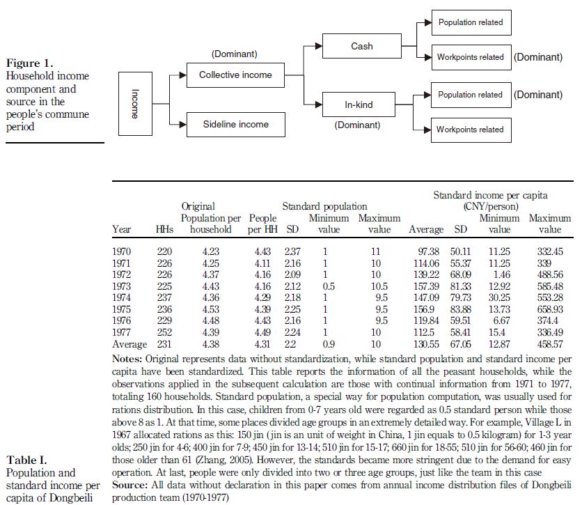
In the age of people’s communes, household income came mainly from two sources: collective income and sideline income. Sideline income – including private fields, breeding, or household handicrafts, were not encouraged and even prohibited when ideology deviated highly to the left. In general, sideline income accounted for no more than 20-30 percent of total household income in that time (Xin, 2000), leaving collective production as the main source of household income.
Income distribution included primary and final distribution. The former, made at the beginning of the year, allocated food, subsidiary food, coal, and other necessities according to household population. The latter was made at the end of the year and was used to balance the difference between work points earned in the year and necessities allocated in the former in terms of cash. Specifically, if cash converted from the work points was more than that from the primary distribution, then the household would get cash from the production team. Otherwise, the household should return or reimburse their cash to the team[3]. In such a turbulent era, the final distribution focused on population more than work points to ensure all households could survive (Xu and Huang, 2014). Final distribution had two determining factors; one was decided by population and the other was decided by work points. The ratio between the two varied: 8:2, 7:3, 6:4, etc. (Zheng, 2010; Huang, 2011; Zhang, 2005). Theoretically, for the factor decided by population, the only determinant was family population – regardless of labor input. In other words, all members in a commune, whether able to work or not, were considered[4]. The principle of counting work points was “more work points, more income.”
In sum, the distribution system in the people’s commune period focused first on all people then on laborers. The ratio of population to laborers can be illustrated as following. If a production team had 10,000 attached China Yuan (CNY) for distributing (net output value in cash after removing cost and tax), then 7,000 CNY would be distributed by total population (suppose the ratio of total population to laborers is 7:3).
In that case, a household with four standard persons (suppose their village has 200 in total) could earn 140 CNY ((4/200) × 7,000) from the population-based distribution. The other 3,000 CNY would be distributed according to work points, which means the household would get 45 CNY from the laborer-based distribution if it earned 600 points among the total of 40,000 ((600/40,000) × 3,000).
In short, household income in the people’s commune period was mainly from the collective, and the major part of collectives’ income was the income in kind related to family population (see Figure 1).
3. Data and methodology
3.1 Data sources and description
All applied data were collected from the original account books of Dongbeili production teams[5] which is located in the Southwest end of Taiyuan Basin and about 120 km from the provincial capital, Taiyuan City, Shanxi Province. The average annual temperature and precipitation there is 10.4°C and 477.2 mm, respectively. The main grain crops include wheat, corn, sorghum and cereal, and the major cash crop is cotton. In 1977, there were 1,717 mu of arable land, 1,146 people and 1.5 mu arable land per capita[6]. The data cover the period from 1970 to 1977 with 160 households having complete contiguous information, which is the calculation basis of income mobility. Abstract of population and household income of Dongbeili is shown in Table I.
After standardization, population per household and standard average income of Dongbeili production team were 4.31 and 130.55 CNY, respectively. The absolute value of income ranked slightly above the domestic average level at that time. Unlike the continuously rising national trend, however, the income per capita of Dongbeili first increased and then decreased, showing an inverted U shape and peaking at 157.39 CNY in 1973. Compared with the value in 1970, income per capita in 1977 had increased by 15.5 percent in 1977. Additionally, individual income differences became bigger when income got higher. For instance, standard income per capita was 156.90 CNY in 1975, when the standard deviation reached the highest value of 83.88 in the sample period. From these simple descriptive statistics, it is found that peasant households got a low and slowly ascending income before the rural reform, and income differences (standard deviation) rose as income went up.
3.2 Methods
The Gini coefficient and Theil index methods are usually employed to measure gaps between the rich and the poor. These two indicators, however, are both static. Studies on income mobility pay more attention to the amount of economic welfare or its variation for a specific individual or social class in a certain period. The indices on measuring income mobility include the Gini mobility index and the transition matrix, etc. This paper adopts the static Gini coefficient and the dynamic income transition matrix as well as the Gini mobility index to measure income differences[7]. In addition, amount and rank mobility of income are both considered in the Gini mobility index.
3.2.1 Gini mobility index. 3.2.1.1 Income level mobility. Income level mobility means changes of income rank determined by income level, i.e., the variation of income position. For example, there are four positions from low to high: A, B, C, and D. Some households were at A in the base period (BP), and changed into B or some other position at the final period. This process is called income level mobility which is related to the ability of individuals or households to move upwards or downwards between different income levels.
The method of Beenstock (2004) is applied in this paper:

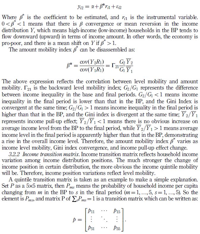
3.2.1.2 Income amount mobility. Income amount mobility means the change of income represented by absolute number or ratio and usually expressed by β convergence or mean reversion.
This paper employs the regression model modified by Wodon and Yitzhaki (2001) and Beenstock (2004):
In terms of the transition mtrix as a whole, the income level will change in a positive direction and the income flows upwards if m < s; the income level will change in the negative direction and the income flows downwards if m > s; while there is no change in income position and no mobility in income if m = s.
Metrics of income transition matrix can be divided into two major categories: the first is relative income mobility indicators (including inertial rates and Shorrocks’s,1978 flow index), and the other is absolute income mobility indicators (non-directional index of Fields and Ok, 1996).
4. Household income mobility in the people’s commune period
4.1 Gini mobility
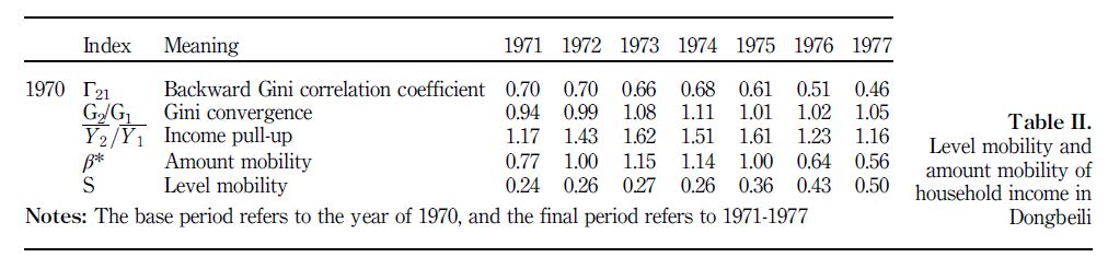
First, it is necessary to calculate household income Gini mobility including level and amount mobility during the people’s commune period. Gini mobility can reflect and disassemble long-term changes of income comprehensively. The income Gini mobility results of Dongbeili production team are shown in Table II.
Income amount mobility was divergent in the short term but convergent in the long term, i.e., income mobility enlarged income difference in the short term, but narrowed it in the long term. Income amount mobility index β* was more than 1 in the short term, showing that amount mobility was divergent in the short term. For example, β* between
1970 and 1974 was 1.14. In the long term, 0 < β* < 1, for instance, the coefficient between 1970 and 1976 was 0.64, demonstrating the existence of β convergence or mean reversion, i.e., high-income households in 1970 tended to flow downwards while low-income ones upwards in the long term. Or in other words, income mobility decreased the income difference by making it more average.
Income level mobility of Chinese rural families had been increasing continuously during this period. First, the value of Γ21 was decreasing gradually. For example, it declined to 0.46 in the 1970-1977 period from 0.70 in the 1970-1972 period, indicating increasing changes in rural household income levels. In other words, mobility grew higher as the correlation between income level in the base and final periods became smaller. Second, level mobility index S rose greatly from 0.24 in the 1970-1971 period to 0.50 in the 1970-1977 period, suggesting growing income mobility as well as less correlation between income level in the final and BPs of Dongbeili.
Generally speaking, the difference between mobility modes of income level and amount would become increasingly smaller if there was no pull-up effect. Such difference would become higher without Gini convergence. Hence, the gap got bigger and bigger with both pull-up effect and Gini convergence. The value of Γ21 and β* were 0.70 and 0.77 in 1970-1971, respectively. The difference between these two modes reflected about 17.1 percent pull-up effect and about 6.08 percent Gini convergence effect. However, Γ21 = 0.46 and β* = 0.56 in the 1970-1977 period, reflecting 15.52 percent pull-up effect and 4.99 percent Gini divergence effect, respectively.
To summarize, as the two indexes measuring income mobility tended to be accelerated, so the long-term effect was beneficial for low-income households. The special distribution system of work points helped low-income households to improve their lives.
4.2 Income transition matrix
The income transition matrix is very effective at analyzing locants of variation within income distribution. Therefore the quintiles transition matrix of income mobility is applied in this paper to investigate the direction and degree of income level mobility. First, the average income of each quintile class is calculated before doing transition matrix. As Table III shows, income level fluctuations at different quintiles were relatively consistent, i.e., first rising then declining, according with the overall tendency. Take the third income quintile income as an example: the average income was 88.98 CNY in 1970, and went up to 132.94 CNY in 1974 before declining to 103.29 CNY in 1977. By comparing all quintiles, the fluctuations became larger as the quintile went higher. The difference of average income at the first quintile was 18.73 CNY between 1974 and 1970, but at the fifth quintile the difference was 99.03 CNY. This means gaps among high-income households were wider than those among low-income ones.
The data of Dongbeili production team is divided into two periods: 1970-1974 and 1974-1977. Income mobility is then calculated for each period respectively. See Table IV for the income transition matrix[8].
As shown in the matrixes, income inertia ratio (immobility ratio) was decreasing gradually (47.6 percent in the BP and 45.8 percent in the final period), demonstrating that relative income mobility was rising. Specifically, 64 percent of those households who were the poorest during 1970-1974 remained at the same level in the final period, and 58 percent of those richest in the BP remained at the same level in the final period. During 1974-1977, only 42 percent of households remained at the poorest level. By comparing the two stages, the mobility of two low-income classes had been strengthening. The ratio of households remaining the same income level was 64 and 36 percent, respectively at the first stage, and declined 42 percent and respectively 29 percent at the later stage. However, income mobility within the third and fourth quintiles was quite the opposite of the first two. The number of household ratios remaining at the original levels grew from 38 to 47 percent in the third quintile, and from 42 to 55 percent in the fourth quintile during the two periods. Having a high number of homes remaining the same level of income indicates that the mobility of these two classes was diminishing. The mobility at the highest quintile experienced minute changes, decreasing from just 58 to 56 percent. The matrixes show that it was easier for low-income households to increase their earnings.
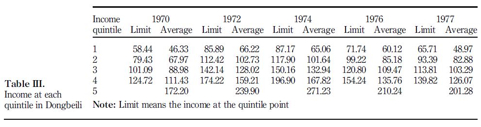
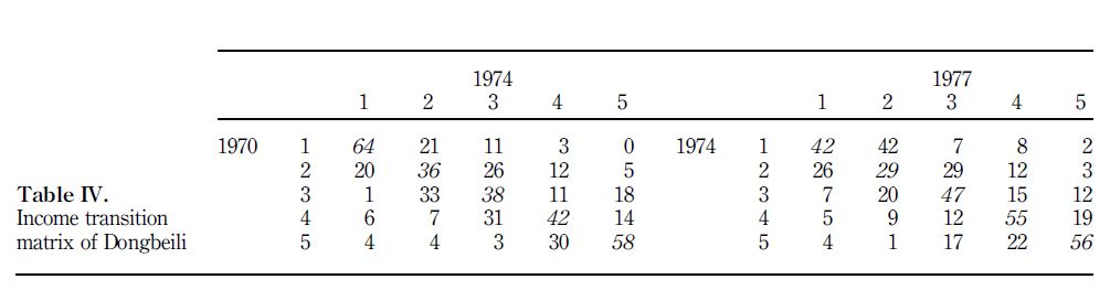
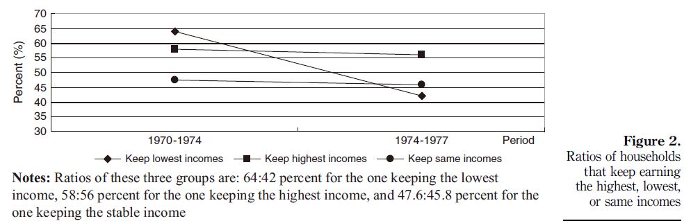
Figure 2 gives a clear view of the income mobility between different groups in the two periods. The low-income group changed the most, and its position as the lowest income declined significantly. Simultaneously, ratios within the highest income quintile experienced a consistent, yet slight decline, proving that income mobility was pro-poor once again.
The other two indexes (Shorrocks flow index and Fields-Ok non-directional index) of income transition matrix showed the same results. Shorrocks flow index was 0.201 in the 1970-1974 period and 0.265 in the 1974-1979 period, demonstrating the whole social mobility was increasing. All the absolute income mobility indexes (Fields-Ok non-directional Index) in the 1974-1977 period were higher than those in the 1970-1974 period. For instance, the aggregate index was 522 in the 1970-1974 period and 532.5 in the 1974-1977 period, while the per capita index was 0.74 in the 1970-1974 period and 0.78 in the 1974-1977 period, and the mobility percentage was 26.99 percent in the 1970-1974 period and 28.19 percent in the 1974-1977 period[9]. To sum up, absolute income mobility became stronger at the end of the people’s commune period, and became more beneficial for low-income earners.
4.3 Correlation between income mobility and inequality
Both of the two major indexes of income mobility (Gini mobility and income transition matrix) demonstrate that income mobility was beneficial for low-income households, i.e, it was pro-poor. At this point, it becomes necessary to identify the relationship between mobility and inequality. It is with confidence that a progress index of long-term income equality defined by Fields (2007) on the basis of Shorrocks (1978) is applied to measure income mobility in terms of the effect from mobility on income inequality. It suggests that the enhancement of income mobility is conducive to narrowing income inequality. Its formula goes as follows:
where G(L) represents the long-term income Gini coefficient meaning average income at the base and final periods; G(F ) represents the short-term income Gini coefficient referring to income level at the BP; E is the inequality degree which means there is no mobility if E = 0, long-term income distribution is more equal than the short term if E > 0, and in that case, the equalization gets stronger as the value of E gets higher, and vice versa. E < 0 means the long-term income distribution is less than that in the short term (see Table V).
Short-term income inequality reflects the income distribution in a single year only, while the long-term one reflects the average income distributions from the beginning to the ending years. Therefore, as long as there is income mobility between each year, long-term income distribution inequality may not be such an issue even if income inequality rises in the short term. Case studies suggest that short-term inequality coefficient is higher than that in the long term. For instance, the short-term inequality coefficient was 0.1951 and higher than the long-term 0.1840 in 1971. Therefore, the inequality degree was lower in the long term.
As shown in Table V, no matter how the long-term and short-term inequality degrees changed independently, the index E always exceeded 0 which meant long-term income distribution was more than that in the short term and income mobility played a more and more important role in the degree of equalization between peasant households (E exceeds 0 and keeps growing). E ascended from 0.0567 in 1970-1971 to 0.1627 in 1970-1977, witnessing a 186.95 percent increase on equalization effect of income mobility, which meant income mobility was very effective to the equalization of income distribution, i.e., it is helpful to narrow the income gap. However, such variation might well be driven by the income growth of poor people when all classes had limited income growth during that period, verifying the findings of Putterman (1993).
5. Factors influencing income mobility
In order to discuss the factors influencing income mobility, or, to find out the elements leading to changes in household long-term income, the authors intend to build a regression model with which the quintile level mobility is divided into three directions (upwards, still and downwards) as explained variables. The values are set as 1, 0, and ?1 for directions of upwards, still and downwards, respectively. For instance, the value should be 1 if a household’s income rises from the third quintile to the fourth or higher. According to the traits of explained variables, the multinominal logit model (MLM) will be applied. This model does not require independent variables in descending order. Its basic thought is to select a result as benchmark and compare all others with it, and finally, conduct a binary logit regression based on the compared results. The premise of the MLM model is that the comparison between different results is not affected by adding or reducing valuing results. The model employed in this paper meets this requirement. Table VI shows the meaning of each variable.
This explained variable shows income position changes. Income amount fluctuations are also studied and used to conduct a robustness test.
Explained variables can be represented in two kinds of indexes: quintile mobility direction (1 for upwards, ?1 for downwards, and 0 for still), and logarithmic growth rate of standard income per capita in the two periods (applied for stability test).

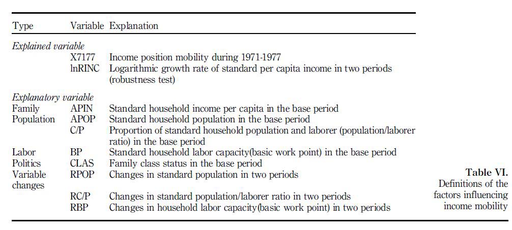
Explanatory variables include family factors in the BP (standard income per capita in the BP), population factors (population quantity, population/laborer ratio), labor capacity factors (basic work point), politics factors (family class status), etc. See Table VII for variables statistics.
5.1 Explained variables
X7177 refers to income quintile change during 1971-1977. The average value is 0.05 indicating more households were growing upwards.
lnRINC7177, an explained variable in linear regression model, refers to logarithmic growth rate of standard income per capita in the two periods.
5.2 Explanatory variables
APIN, which represents age-adjusted standard income per capita in the BP, is the major variable for household income mobility as laborers’ income expectation in the later period is influenced by their income in the BP. In 1971, the average value of APIN was 114.1 CNY in 1971 and slightly declined to 112.5 CNY in 1977.
APOP and C/P represent the standard population and the population/laborer ratio, respectively. They are important factors influencing household income mobility. Generally, the more people being supported in a family, the higher the labor pressure. APOP increased from 4.1 in 1971 to 4.5 in 1977, and C/P increased from 2.3 in 1971 to 2.6 in 1977.
BP is the household basic work point per labor in the BP. In general, higher BP means stronger labor capacity in a household. If two households have the same population structure, the one with higher BP is likely to earn more[10]. In order to eliminate the population effect, male and female labors are set as 1 and 0.8, respectively and mean values are obtained through weighting[11]. BP declined from 8.7 in 1971 to 6.6 in 1977.
Class status is a special variable in the people’s commune period and can be divided into landlord, rich peasant, upper-middle peasant, middle peasant, low-middle peasant, and poor peasant categories. Generally, landlord wand rich (sometimes even upper-middle) peasants were regarded as bad classes who were always discriminated during production and distribution processes in production teams. Therefore, it needs to define a dummy variable.
CLAS to describe class difference. CLAS = 0 for low-middle and poor peasants, and CLAS = 1 for other classes.
RPOP7177, RC/P7177, and RBP7177 refer to changes in standard population, population/laborer ratio, and household basic work point in the two periods, respectively.
Descriptive statistics show that population and the population/laborer ratio increase by 0.38 and 0.22, respectively, but basic work point declines by 4.03.
See Table VIII for mobility direction as explained variables. Comparing 1971-1974 with 1974-1977, the number of still households was greater than that of upward or downward households. In the meantime, the number of upwards households was greater than that of downwards. For instance, still, upwards, and downwards households accounted for 50.3, 25.9 and 23.8 percent, respectively during 1971-1974. In 1974-1977, there were more households flowing up or down than that in 1971-1974. The percentage of still households in the short term was 50.3 percent while in the long term it was 39.0 percent, indicating higher mobility in 1974-1977.
See further MLM estimations in Table IX[12].
The estimation results reveal there was a significant negative correlation between upward income mobility and standard income per capita (APIN) in the BP, demonstrating that it was hard for households with high income to flow upwards. On the contrary, the lower the APIN was, the higher the probability of upward mobility.
Hence, it can be seen that during the people’s commune period, household income was characterized by the pro-poor mobility which was beneficial for low-income earners.
Household population (APOP) has no significant influence on income mobility, while population/laborer ratio (C/P) is a major affecting factor, with its influence on households flowing upwards and a significance at the 5 percent level both in 1971-1974 and 1971-1977. At the same time, the negative effect of C/P on income mobility indicates that families with high dependents/workforce ratio tended to be lacking on income upward mobility, which accords well with the history of the people’s commune. At that time, households enjoying the highest degree of prosperity were usually those with more laborers and less consumers, while those with more consumers and less laborers tend to overspend.
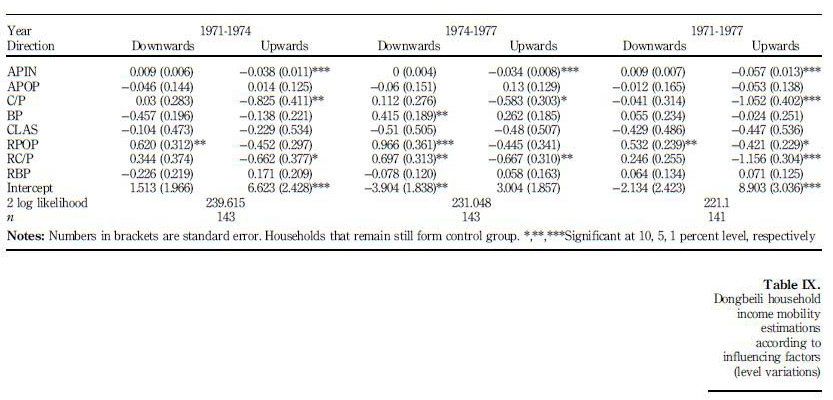
Standard household work points in the BP had little influence on income mobility and only showed a significant positive correlation with households flowing downwards during 1974-1977. This suggests that the income of families with a greater number of work points are more susceptible to economic decline. It also proves that labor quality limited or no effect on income mobility. On the other hand, an explanation for the inverse of this might be that some laborers stopped working due to population structure changes and capacity was lowered. Changes in household basic work points in the two periods (RBP) had no obvious influence in determining income mobility.
Class (CLAS) showed no significant effect throughout the period, proving that social status had no effect on household income along with its mobility at the end of the people’s commune period.
Change in standard population in the two periods (RPOP) had an apparent influence on income mobility – especially on those flowing downwards. Increases in total population were not conducive to upward income flow for rural households. This is further affirmed by changes in the population to laborer ratio (RC/P).
In summary, household income mobility was mainly influenced by population structure and income per capita in the BP. The effect that population structure had is
shown through the population/laborer ratio. It was difficult to achieve upward flowing income when the dependents to laborer ratio was high. While basic work points and social status had little influence on income mobility, household income in the BP was of greater significance when determining the ability for upward mobility.
In order to fully appreciate the importance of the results, income amount changes in the two periods are calculated (see Table X). Estimation results based on income amount changes are similar to those based on level changes, proving the robustness of estimations.

6. Conclusions
This paper studied the long-term income differences of rural households during the people’s commune period based on income distribution files of the Dongbeili production team in Shanxi Province. The distribution system at that time revealed that household income came mainly from production teams, and without them, peasants would likely not have survived had they not relied on the collectives.
Through this study of income mobility, it was found that both the amount of wealth increase and the level of mobility between income groups in the long term were more than those in the short term, and that the long-term income mobility results were pro-poor. The income transition matrix also showed that income mobility was beneficial for poor people to improve their status, for their income growth was faster than that of rich people. In addition, a detailed calculation on the correlation between income mobility and inequality also demonstrates that income distribution in the long term was more equal than that in the short term, and the effect of equalization was becoming increasingly powerful.
Among the factors influencing income mobility, the most important one was population structure[13], i.e., population/laborer ratio, instead of labor input. When this ratio was low, it was easy to increase income. Neither basic work point nor social status had significance.
Finally, it is meaningful to discuss why the people’s commune system failed. As stated in the introduction of this paper, there are various explanations for this issue, and research findings in this paper may be of particular interest when attempting to understand it. Household income mobility demonstrates that household income gaps were relatively small in the people’s communes, i.e., the degree of equality was very high. Additionally, the major factor affecting income mobility was family population rather than the acquirement of basic work points. It is arguably the case that this fact was the single most important reason in determining why work enthusiasm at the time was so low. We will give detailed demonstration on this point in another paper. The biggest contribution of this study is to analyze the differences of peasant households in the people’s commune in detail with a totally new angle and unique data, which is expected to build solid foundation for following researches and to provide reference for today’s agricultural policies.
Compared with now and the period of people’s commune, the institutional environment that affected income mobility has already changed. Specifically, in the people commune period, the labor factor was suppressed while the factor of household structure was over- weighted, which eroded the incentive to farmers; by contrast, the current factors influencing income mobility have changed from the purely demographic factor to human capital, material capital, and employment (Shi et al., 2010; Yan et al., 2014), which is conducive to stimulate enthusiasm for labor. Therefore, the development of China’s agricultural policy should keep its direction of reform.
Notes
1. For existing research on income differences in people’s communes, refer to the insightful comments by Putterman (1993) and Griffin and Saith (1981).
2. It will be the topic of our next study that how mobility of farmers’ income affects efficiency of the people’s commune.
3. When a household had no cash, its debt would be recorded to be repaid the next year.
4. Of course, the part decided by population was also compensated by work points. Standard conversion was made according to age: for instance, children under three years old were converted as 0.5 standard person, four to seven-years-old as 0.8 standard person, etc. (Zhang, 2005; Xin, 2005).
5. See Huang (2012) for a description of production team account book.
6. mu is a unit of area, 1 mu approximately equals to 0.16 acre.
7. The construction of the research method of this study is mainly benefited from Shi et al. (2010), the authors hereby acknowledge Shi and her partners.
8. Results in this paper have been simplified. Please contact the author for more details.
9. Due to limited paper length, detailed index results are omitted. For complete calculation results, please contact the author.
10. It is a complicated process to evaluate basic work point. Many factors including work ability, age, attitude, gender, and class are considered. This index can reflect real labor quality basically (Zhang, 2005).
11. In people’s commune, male basic work point is 10 and female 8 (Zhang, 2005).
12. Highest income households cannot flow upward and lowest cannot flow downwards.
To solve this problem, we divide household income into decile groups, remove the first and tenth groups, and make regression again. The results are basically the same.
13. There have been some articles that find obvious correlation between household life cycles and income during people’s commune (Huang et al., 2013).
References
Beenstock, M. (2004), “Rank and quantity in the empirical dynamics of inequality”, Review of Income and Wealth, Vol. 50 No. 4, pp. 519-541.
Conn, D. (1982), “Effort, efficiency, and incentives in economic organizations”, Journal of Comparative Economics, Vol. 6 No. 3, pp. 223-234.
Dong, X. and Dow, G.K. (1993), “Monitoring costs in Chinese agricultural teams”, Journal of Political Economy, Vol. 101 No. 3, pp. 539-553.
Feng, H. and Li, Z. (1993), “Study on capital accumulation provided to industry by agriculture in China”, Economic Research Journal, Vol. 9, pp. 60-65.
Fields, G. (2007), “Income mobility”, Working Papers No. 07/19, Cornell University ILR School, Ithaca.
Fields, G. and Ok, E. (1996), “The meaning and measurement of income mobility”, Journal of Economic Theory, Vol. 71 No. 3, pp. 349-377.
Griffin, K. and Saith, A. (1981), Growth and Equality in Rural China, Koon Wah Printing Pte. Ltd, Singapore.
Hsiung, B. and Putterman, L. (1989), “Pre- and post-reform income distribution in a Chinese commune: the case of Dahe Township in Hebei Province”, Journal of Comparative Economics, Vol. 13 No. 3, pp. 407-445.
Huang, S., Sun, S. and Gong, M. (2005), “The impact of land ownership structure on agricultural economic growth: an empirical analysis on agricultural production efficiency on the Chinese Mainland”, Social Sciences in China, Vol. 3, pp. 38-47.
Huang, Y. (2011), Rural Labor Work under Work-Point System, China Agriculture Press, Beijing.
Huang, Y. (2012), “Review on rural economic distribution files in the collectivization Era Zutang production team of Jiangsu as a case”, Ancient and Modern Agriculture, Vol. 4, pp. 14-24.
Huang, Y., Yongwei, C. and Jun, L. (2013), “Household income in rural collectivization: the effect of life cycle”, Researches in Chinese Economic History, Vol. 2, pp. 36-44.
Huang, Z. (2000), Peasant Family and Rural Development in the Yangtze Delta, Zhonghua Book Company, Beijing.
Kung, J. (1993), “Transaction costs and peasants’ choice of institutions: did the right to exit really solve the free rider problem in Chinese collective agriculture?”, Journal of Comparative Economics, Vol. 17 No. 2, pp. 485-503.
Kung, J. (1994), “Egalitarianism, subsistence provision, and work incentives in China’s agricultural collectives”, World Development, Vol. 22 No. 2, pp. 175-187.
Li, H. (2010), Village China under Socialism and Reform: A Micro-History, Law Press·China, Beijing.
Lin, J. (1988), “The household responsibility system in China’s agricultural reform: a theoretical and empirical study”, Economic Development and Cultural Change, Vol. 36 No. 4, pp. 199-224.
Lin, J. (1990), “Collectivization and China’s agricultural crisis in 1959-1961”, Journal of Political Economy, Vol. 98 No. 6, pp. 1228-1252.
Putterman, L. (1990), “Effort, productivity, and incentives in a 1970s Chinese people’s commune”, Journal of Comparative Economics, Vol. 14 No. 1, pp. 88-104.
Putterman, L. (1993), Continuity and Change in China’s Rural Development: Collective and Reform Eras in Perspective, Oxford University Press, New York, NY.
Shi, X., Alex, N. and Xian, X. (2010), “Household income mobility in rural China: 1989-2006”, Economic Modelling, Vol. 27 No. 5, pp. 1090-1096.
Shorrocks, A. (1978), “Income inequality and income mobility”, Journal of Economic Theory, Vol. 46 No. 2, pp. 376-393.
Sun, S. (2009), “Economic development and relation between the industry and agriculture sectors: the Chinese planning economy revisited in cliometrics”, Economic Research Journal, Vol. 8, pp. 135-146.
Sun, S. and Liu, X. (2014), “Institutional change, elements misplaced and efficiency loss – an empirical analysis of China agricultural cooperative movement”, working paper, Shandong University, Jinan.
Wen, G. (1993), “Total factor productivity change in China’s farming sector: 1952-1989”, Economic Development and Cultural Change, Vol. 42 No. 2, pp. 1-41.
Wodon, Q. and Yitzhaki, S. (2001), Growth and Convergence: An Alternative Empirical Framework, World Bank and Hebrew University, Washington DC and Jerusalem.
Wu, L. (2001), “1949-1978 China ‘scissors difference’ differentiation”, Researches in Chinese Economic History, Vol. 4, pp. 3-13.
Xie, S. (2006), “Study on village economy under people’s commune system – focus on ‘notice’ interpretation”, Researches in Chinese Economic History, Vol. 2, pp. 79-87.
Xin, Y. (2000), “The study on family’s sideline in rural people’s commune”, Historical Research of Communist Party of China, Vol. 9.
Xin, Y. (2005), “Research on rural distribution system in people’s commune”, History of Communist Party of China Press, Beijing.
Xu, W. and Huang, Y. (2014), “The materialization and affection of household labor reward on people’s commune era: the case of production team in Hebei Province (1970s)”, Researches in Chinese Economic History, Vol. 4, pp. 168-174.
Yan, B., Zhou, Y. and Yu, X. (2014), “A study on household income mobility in rural China from 1986 to 2010”, China Economic Quarterly, Vol. 13 No. 3, pp. 939-968.
Yao, Y. and Zheng, D. (2008), “Heavy industry and economic development: the Chinese planning economy revisited”, Economic Research Journal, Vol. 4, pp. 26-36.
Zhang, J. (2007), “Labor incentive and inefficiency of collective labor under the work points system”, Sociological Studies, Vol. 5, pp. 2-11.
Zhang, L. (2005), Farewell, My Ideal – Research on People’s Commune System, Shanghai People’s Publishing House, Shanghai.
Zheng, W. (2010), “Distribution system and population growth in the collectivization period – the case of Dong Village in Rizhao City (1949-1973)”, Open Times, Vol. 5, pp. 103-114.
Zhou, Q. (1995a), “Reform in China’s countryside: changes to the relationship between the state and ownership (first part)”, Management World, Vol. 3, pp. 178-200.
Zhou, Q. (1995b), “Reform in China’s countryside: changes to the relationship between the state and ownership (first part)”, Management World, Vol. 4, pp. 147-170.
Further reading
Kung, J. and Putterman, L. (1997), “China’s collectivisation puzzle: a new resolution”, Journal of Development Studies, Vol. 33 No. 6, pp. 741-763.
National Bureau of Statistics of China (1982), China Statistical Yearbook 1981, China Statistics Press, Beijing.
Corresponding author
Jun Li can be contacted at: sirlijun@126.com
Received 30 November 2015
Revised 21 April 2016
Accepted 13 June 2016
关键词:现代经济史;农村;收入变动;人民公社;生产队;工分制